User Manual
The program uses two windows, the main control GSLab window and the Image window. The GSLab window features a top panel displaying the phasor plot and a bottom panel organized into seven tabs, each providing access to specific functionalities. The Image Window is dedicated to rendering all images loaded into the software.
Phasor Plot panel
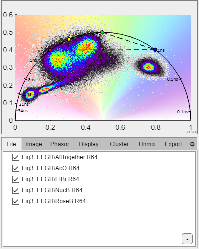
GSLab window and Image window.
This is the main panel where phasor plots are displayed. Hovering the mouse over the phasor space will show a circular cursor the size of which is controlled by the mouse scroll. The central coordinates of the current cursor location are displayed on the top left. If a file is loaded, the pixels whose phasor transform is within the cursor limits will be rendered in the color of the cursor. If the user clicks on the phasor space the cursor position is fixed and a new cursor with a different color is used as mouse pointer. If one or more cursors are on the phasor plot a button with a red X appears in the top-right corner that clears all cursors on the phasor plot.
File tab
Loaded files are listed in the main panel. The checkboxes in front of each file name allow the user to include/exclude each loaded file from the representation and analysis.
Contextual menu options (right-click):
Calibration File: Sets the selected file as calibration. Will obtain the photon weighted average coordinates of the phasor distribution and assign it the lifetime in the Calibration Lifetime box in the Calibration Panel.
Load menu:
Tif Sequence: prompts user to select tiff file(s).
FLAME raw: prompts user to select a folder containing raw FLAME images.
Leica FALCON SnG: prompts user to select a folder containing trios or quartets of tifs exported from the Leica Falcon as S and G coordinates using Save phasor GS - Fixed Range in LASX. The steps are:
1. In the LAS X FLIM/FCS window, select the Intensity tab above the images.
2. In the FLIM tab on the left menu, at the bottom there is a Save Image button.
3. Click that and the Save Image window opens:
4. Select Tiff tab.
5. Select checkbox Save Phasor GS.
6. Select the radio button Fixed Range.
7. Set the Factor or Range to per Grey Level and input 1 in the edit field box.
Zeiss lsm: prompts user to select Zeiss lsm file(s).
FLIM LABS json: prompts user to select FLIM LABS json file(s).
PicoQuant ptu: prompts user to select ptu file(s). Requires Python with C.Gohlke's ptufile library [GitHub].
Becker & Hickl sdt: prompts user to select sdt file(s). Requires Python with C.Gohlke's sdtfile library [GitHub].
SimFCS ref: prompts user to select ref or r64 file(s).
Trace txt/csv: prompts user to select txt or csv files with single traces.
Saved Session: loads a previously saved session including files and settings
Save menu:
SimFCS ref: generates a phasor coordinates file with the first two harmonics.
Current session: prompts user to browse location and input file name to save current settings and paths to loaded files.
Move:
Top/up/down/bot: Moves the selected file to the desired position in the list to change the arrangement in the display window and in exported images.
Odd/even: Moves all files to split the current list into two halves taking alternating items from list.
Check All/None/Invert/Alternate: Checks all or none or inverts or alternated checked files from the list for their display and analysis.
Emphasis:
Selected: Opens color picker to depict phasor data for selected file.
Checked: Opens color picker to depict phasor data for all checked files.
None: Removes emphasis on files and plots all together in a single density colormap.
Clear All/Unchecked: Removes all or unchecked files from memory.
Calibration Panel button: folds/unfolds the calibration panel.
Apply checkbox: apply the current calibration to the loaded files or not.
File/Manual radio button: allows the user to set calibration based on selected files or on manual input.
File mode: The calibration panel table appears with three columns:
The first column is the text tag of the calibration file. By default it is All meaning all files, if user changes that to a specific text string, only files whos name contains the specified string will be calibrated using the selected calibration file.
The second is the lifetime associated with the file. This value can be changed by the user.
The third is the filename that was used for the calibration.
Manual mode: Two boxes appear:
Phase shift: applies the inputted phase shift to the data (in radians).
Modulation factor: applies the inputted modulation factor to the data(normalized to unity).
Calibration Lifetime box: User can input the lifetime of the next file that is to be set for calibration.
Clear button: clears all calibration files.
Image tab
This tab contains the image manipulation parameters and settings for rendering the intensity images prior to phasor transform.
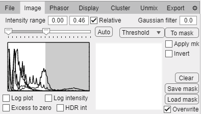
Image tab.
Intensity threshold input boxes: set intensity lower and upper bounds for image rendering.
Slide bar also sets the lower and upper bounds for image rendering.
Relative checkbox: indicates if the intensity values are relative to the dynamic range of each file or are the thresholds are to be set in absolute intensity units.
Auto button: Automatically set the range to a percentile of the data (determined by user preferences).
Intensity histogram panel shows the intensity histogram of each loaded file.
Log plot checkbox: plot the intensity histogram in logarithmic scale. This option is useful when you have pixels with low counts and others with very high counts.
Log intensity checkbox: Render images in logarithmic intensity to compensate high dynamic range images.
HDR intensity checkbox: Render images using a pixel-wise local dynamic range to compensate high dynamic range images.
Excess to zero checkbox: Excludes pixels that are being saturated by the upper bound of the intensity thresholding.
Gaussian filter text box: Apply a gaussian filter to images of the input size in pixels.
Threshold/cursors dropdown:
Threshold: masks will be created based on intensity thresholds.
Cursors: masks will be created based on cursors set on the phasor plot.
To mask: Create a mask using the dropdown selection.
Apply mask checkbox: Apply or not the current mask to the loaded data.
Invert checkbox: Invert the current mask.
Clear: Delete current mask.
Save mask button: Save current masks to file (png if single file or stacked tiff if multiple files).
Load mask button: Load image to use as binary mask. If a single image is loaded it will be applied to all files loaded, if a multislice tiff is loaded, each slice will be sequentially applied to each loaded image. Images created in other softwares can be uploaded and used to exclude pixels from phasor analysis. Additionally if an image with integer labels can be loaded and it will be treated as region labels to export average region phasor data (Export tab - Masked object data checkbox)
Overwrite: Ovewrite current mask when loading or apply loaded mask on current mask.
Phasor tab
The phasor tab includes all parameters affecting the phasor transform computation and the associated measurements.
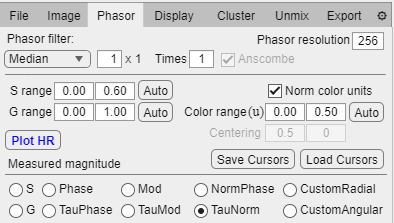
Phasor tab.
Phasor filter dropdown: Set the filter type, one of median or a wavelet family (requires Wavelet Toolbox).
Phasor filtering box: Set the size of the median filter kernel or wavelet support (for Daubechies and Symlets).
Wavelet support dropdown: Set the support of the selected wavelet family (requires Wavelet Toolbox).
Times box: Number of times the filter should be applied.
Level box: Wavelet denoising level (requires Wavelet Toolbox).
S range boxes: Lower and upper limits of the S axis for displaying the phasor plot.
Auto button: Automatically set the S axis limits to a percentile range (determined by user preferences).
G range boxes: Lower and upper limits of the G axis for displaying the phasor plot.
Auto button: Automatically set the G axis limits to a percentile range (determined by user preferences).
Color range boxes: Lower and upper limits for the color range (in units of a whole turn for angular quantities and in phasor units for radial quantities).
Norm color units: Toggle between setting the color range in units over unit circle or in the selected magnitude units.
Auto button: Automatically set the color range to a percentile range (determined by user preferences).
Centering boxes: G and S coordinates of the center of a custom measuring magnitude.
Phasor resolution box: Number of bins to use in the phasor space for computing the phasor plot.
Plot HR button: Compute phasor plot for High resolution images.
Save Cursors button: Save the current cursor position, dimensions and colors in a file.
Load Cursors button: Load a file containing cursor positions, dimensions and colors.
Measured Magnitude radio buttons:
S: Generate a color gradient based on S coordinate.
G: Generate a color gradient based on G coordinate.
Phase: Generate a color gradient based on polar phase.
TauPhase: Generate a color gradient based on polar phase and compute the associated lifetime.
Mod: Generate a color gradient based on polar modulation.
TauMod: Generate a color gradient based on polar modulation and compute the associated lifetime.
NormPhase: Generate a color gradient based on pseudo-phase.
TauNorm: Generate a color gradient based on pseudo-phase and compute the associated lifetime.
CustomRadial: Generate a custom radial color gradient (center coordinates need to be specified).
CustomAngular: Generate a custom angular color gradient (center coordinates need to be specified).
Display tab
The display tab includes all options that are related to phasor plot style and formatting.
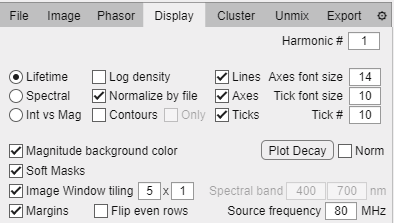
Display tab.
Harmonic # numeric box: Plot the phasor in the corresponding harmonic number (if higher than 1 it will show in red as a warning).
Phasor style radio button:
Lifetime: Sets the S and G ranges appropriate for lifetime phasor and adds universal circle lines.
Spectral: Sets the S and G ranges appropriate for spectral phasor and removes universal circle lines.
Int vs Mag: Will substitute the phasor plot for a histogram of pixel intensity versus phasor magnitude (using the value in the radio button in the Phasor tab).
Log density checkbox: Plot phasor density in log scale enhancing bins with low counts.
Normalize by file checkbox: The phasor distribution density range of each loaded file is normalized so all files appear in similar color range regardless of the spreading of the data.
Contours checkbox: Adds contour lines for lower counts in the phasor plot.
Only checkbox: Removes heatmap so phasor plots are only contour.
Lines checkbox: Draws the universal semicircle for lifetime or the unity circle for spectral.
Axes checkbox: Depicts axes G and S units.
Ticks checkbox: Adds ticks of selected lifetimes/wavelengths depending on excitation source frequency/spectral band.
Axes font size box: Choose the font size for the S and G axes.
Tick font size box: Choose the font size for tick values displayed.
Tick # box: Choose the nuber of ticks to display.
Magnitude background color checkbox: Plot the color gradient according to the measured magnitude selected in the Phasor tab.
Soft masks checkbox: Overlays cursor/magnitude colors on the intensity window as a soft mask (colored intensity image) or hard mask (just the colors regardless of intensity).
Image window tiling checkbox: Force tile arrangement in the intensity window.
Image window tiling numeric boxes: Set the number of rows and columns for displaying the loaded files.
Margins checkbox: Add/remove margin between images in the intensity window.
Flip even rows checkbox: Arranges tiles in zig-zag to account form some mosaic stage paths.
Source frequency numeric box: Set the lifetime excitation laser frequency for the phasor transform trigonometric period (only for lifetime display mode).
Spectral band numeric boxes: Set the spectral limits in nm for the spectral phasor transform (only for spectral display mode).
Plot Decay button: Plot the temporal/spectral curve for each file.
Norm checkbox: Normalize plots to maximum value.
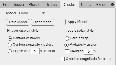
Cluster tab
The clustering tab is used to create automated clustering of phasor distributions in the phasor space.
Cluster tab.
Model dropdown: Select clustering model (currently only GMM).
Train model: Taking the data on the phasor plot, a gaussian mixture models is trained using the expectation-maximization algorithm. The user must select the number of clusters to model by the starting locations of the clusters.
Clear model: Clears the current trained model.
Apply model: Re-applies the model to the current displayed data.
Phasor display style:
Contour of model: Plots the agglomerated sum of gaussians as a single contour plot.
Contour separate clusters: Plots each clusters gaussian component as a separate contour plot.
Ellipse with percentage of data: Plots a single contour for each gaussian such that it contains the percentage of the data set by the text box.
Image display style:
Hard assign: Each pixel is colored with the gaussian component that has a higher posterior probability.
Probability assign: Each pixel is colored with a linear combination colors corresponding to the linear combination weights of each gaussian component in the pixel.
Blending percentage: Applies smoothing to the color masking image to blend regions.
Override magnitude for export: If checked it will swap the magnitude-colored checkboxes in the export tab for GMM-colored checkboxes in order to allow user to export the resulting images of the clustering.
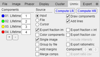
Unmix tab
This tab includes all options for defining pure components to run the multi-harmonic multi-component phasor unmixing routines.
Unmix tab.
Compute LR button: Computes unmixing and generates the selected exporting options using the low resolution versions of the loaded images.
Compute HR button: Computes unmixing and generates the selected exporting options using the high resolution versions of the loaded images.
Source radio buttons:
Manual: Use the Components panel to manually typed in lifetimes of pure single-exponential components for the unmixing.
File: Select loaded files as empirical components for the unmixing.
Cursors: Use point-and-click cursors as components (allows up to 3 components because of harmonic limitation)
Components panel: (Manual mode).
(+/-) buttons: Add/remove a component for the unmixing.
Colored circle button: Open up the color palette to select the color assigned to the component.
Lifetime numeric box: Input the lifetime of the component.
Components panel (File mode): The loaded files list is shown and individual files can be checked to use as a empirical component. The photon-weighted average phasor coordinates is computed for each checked file and the color selected in the manual component panel is assigned to each file.
Draw components checkbox: Plots the position of the unmixing components.
Add lines checkbox: Draws lines between consecutive components in the phasor plot.
Export fraction im. checkbox: When enabled exports each component as an image and raw data in different formats:
Color components checkbox: Export fractional intensity images based on the color selection in the components panel.
Single Image checkbox: Groups into a single image the output of the unmixing instead of individual images for each file and each component separately (uses tiling rows/columns in Display tab).
Group by file checkbox: Creates a single image with all the components for each file or creates a single image for all the files for each component (uses tiling rows/columns in Display tab).
Add margins checkbox: Adds/removes margin between the tiles in the composed images.
Merge components checkbox: Creates a merge image based on the color selection of the components tab (option enabled when Group by file is unchecked).
Export fractions x int: Export the photon fraction images as absolute number of photons assigned to each component (normalized to the dynamic range of the 8-bit output image) or as relative fractions over unity (again, normalized to the dynamic range of the 8-bit output image).
Export fraction csv checkbox: The calculated fractional intensity values of all pixels surviving thresholds is exported as a spreadsheet, one column per component.
Include intensity checkbox: Adds the intensity values for each pixel as the first column of the exported csv file (only available when Export fraction csv is checked).
Export ratiometric checkbox: Computes a ratiometric image using two components X/(X+Y).
Component numeric boxes: Select the component X and Y for ratiometric imaging.
Export ratio csv checkbox: Export a spreadsheet of pixel calculated ratiometric values.
Export tab
Options regarding exporting of images and data files.
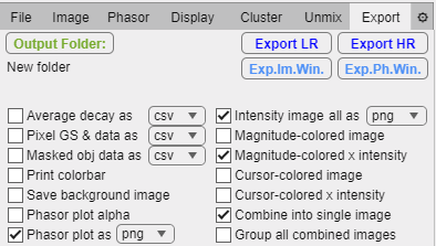
Export tab.
Output Folder button: Prompts user to select a path to a folder where data should be saved. The folder name is displayed below.
Export LR button: Export data using the low-resolution downsampled images for faster computational time.
Export HR button: Export data using the original resolution images.
Exp.Im.Win button: Export the current image window contents as an image.
Exp.Ph.Win button: Export the current phasor plot panel as an image.
Data export options:
Average decay as checkbox: For each checked file generate a file with the average intensity in each spectral/lifetime channel.
Decay as dropdown: Select the file format.
Pixel GS & data as checkbox: For each checked file generate a file with the phasor coordinates and all phasor magnitudes.
Pixel GS & data as dropdown: Select the file format.
Masked obj data as checkbox: If a mask is loaded, detect all objects based on pixel connectivity (8) and obtain mean values for each detected object.
Masked obj data as dropdown: Select the file format.
Print colorbar checkbox: Render a colorbar of the measured magnitude color gradient
Save background image checkbox: Render a color gradient corresponding to the measured magnitude on the phasor plot.
Phasor with axes checkbox: Export the phasor plot with the axes numbers and ticks.
Phasor plot alpha checkbox: Export phasor plots as png files with transparency (only if exported separately).
Phasor plot as checkbox: For each checked file export its phasor plot.
Phasor plot as dropdown: Select the file format for phasor plots.
Intensity image checkbox: For each checked file export its intensity image in grayscale.
Intensity image all as dropdown: Select file format for image exports.
Magnitude-colored image checkbox: For each checked file export the magnitude-colored image (hard mask style).
Magnitude-colored x intensity image checkbox: For each checked file export the magnitude-colored image times the intensity image (soft mask style).
Cursor-colored image checkbox: For each checked file export the cursor-colored image (hard mask style).
Cursor colored x intensity image checkbox: For each checked file export the cursor-colored image times the intensity image (soft mask style).
Combine into single image checkbox: For each checked file join all selected exports into a single file (it will override the phasor plot file format if selected).
Group all combined images checkbox: Join all file exports into a single image using the Image Window tile disposition.
Preferences (⚙) tab
General options for GSLab operation.
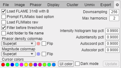
Preferences tab.
Load FLAME 31nB with B checkbox: Load the blue channel as a separate file.
Prompt FLIMlabs load oprion checkbox: Prompt user when loading FLIMlabs json if raw or precalibrated data should be loaded.
Load FLIMlabs raw checkbox: Load FLIMlabs json as raw data ignoring precalibrated phasor coordinates.
Filter before threshold checkbox: Apply filter before or after thresholding the image.
Add folder to the name: Files in File tab are listed including the folder name where the files are in the host machine.
Downsampling box: Size of low-resolution images. Set to 0 for no downsampling.
Max harmonics box: Set the number of harmonics to compute when loading data.
Density colormap dropdown: Allows choices of different color schemes for the phasor density heatmap (if last option single color is selected the button to select color is enabled).
Magnitude colormap: Allows choices of different color schemes for the phasor-based measurement (if last option single color is selected the button to select color is enabled).
Cursor colors panel: Each colored button corresponds to the successive cursors that can be used, click on the buttons to open the color palette and change the color of the cursor.
Intensity histogram top pctl: Set the percentile to cut when normalizing (Image tab - relative checkbox) and when depicting the intensity histogram.
Autointensity pctl: Set the percentile of data to include when using the auto range button (Image tab).
Autocoord pctl: Set the percentile of data to include when using the auto G and S buttons (Phasor tab).
Autointensity pctl: Set the percentile of data to include when using the auto color button (Phasor tab).
UI color button: Set the general color tone of the user interface.
Dark mode checkbox: Set the interface to dark mode.
Update: Download latest version (not available for Windows deployed version).
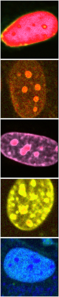
Image Window
The Image Window contains the rendered images. Hovering over an image in this window will select the respective file name in the file tab and will display a black cursor on the phasor plot marking the phasor coordinates of the pixel under the mouse pointer.